Distinguishing introductions from local transmission
Simon Frost
University of Cambridge, and the Alan Turing Institute


A matter of scale
- Infectious diseases know no borders
- Large populations with few introductions
- May be heterogeneous
- May require extensive computation to simulate
- Limited data
- Small subpopulations may be more homogenous, with more comprehensive data, and be faster to simulate
- Have to consider introductions from outside
Sources of infection
- Infections observed in a specific population may result from:
- Infected individuals moving into the population
- Individuals becoming infected from someone outside the population
- Local transmission between members of the population
- Within a population, there are those who do and do not contribute to onward transmission
Why do we care?
- Mistaking introductions for local transmission may lead to underestimates of \(R_0\)
- Critically affects interpretation of local intervention strategies
- Relative size of imports and local transmission affects global disease persistence
How can we distinguish?
- Using case onset data
- Simple observation may suffice
- Imports may result in a different dynamic pattern
- Using genetic data
- Additional epidemiological data
- Contact tracing data
- Subpopulation membership
Epidemiological contexts
- Recurrent zoonoses
- e.g. influenza H7N9, Lassa fever,…
- School outbreaks of measles
- HIV
- Introductions are important due to the long asymptomatic, infectious period
- Dependent on the rate of introductions:
- If low, then rather limited data may be sufficient to infer the source
- If high, then more data/complex models are needed
RSV in households in coastal Kenya
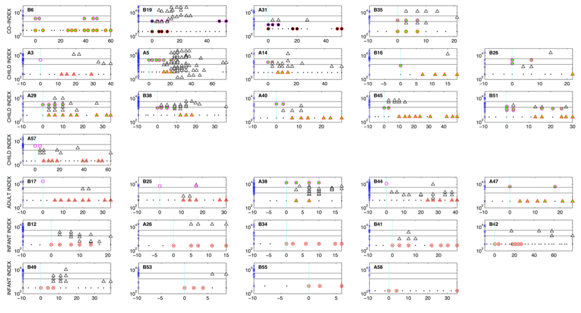
Munywoki et al. J Infect Dis (2013)
RSV in households in coastal Kenya
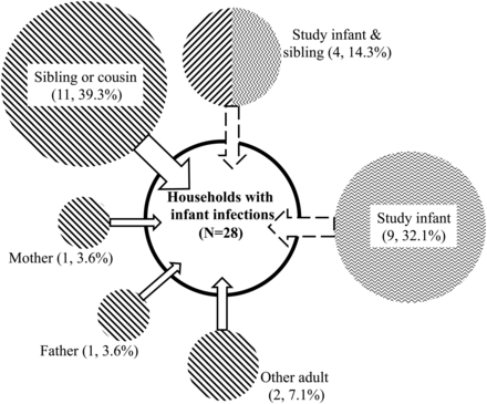
Munywoki et al. J Infect Dis (2013)
Origin of Ebola epidemic in W. Africa
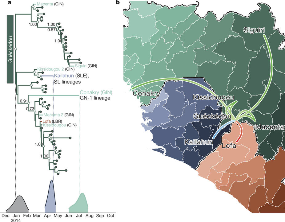
Dudas et al. Nature (2017)
Norovirus in a hospital
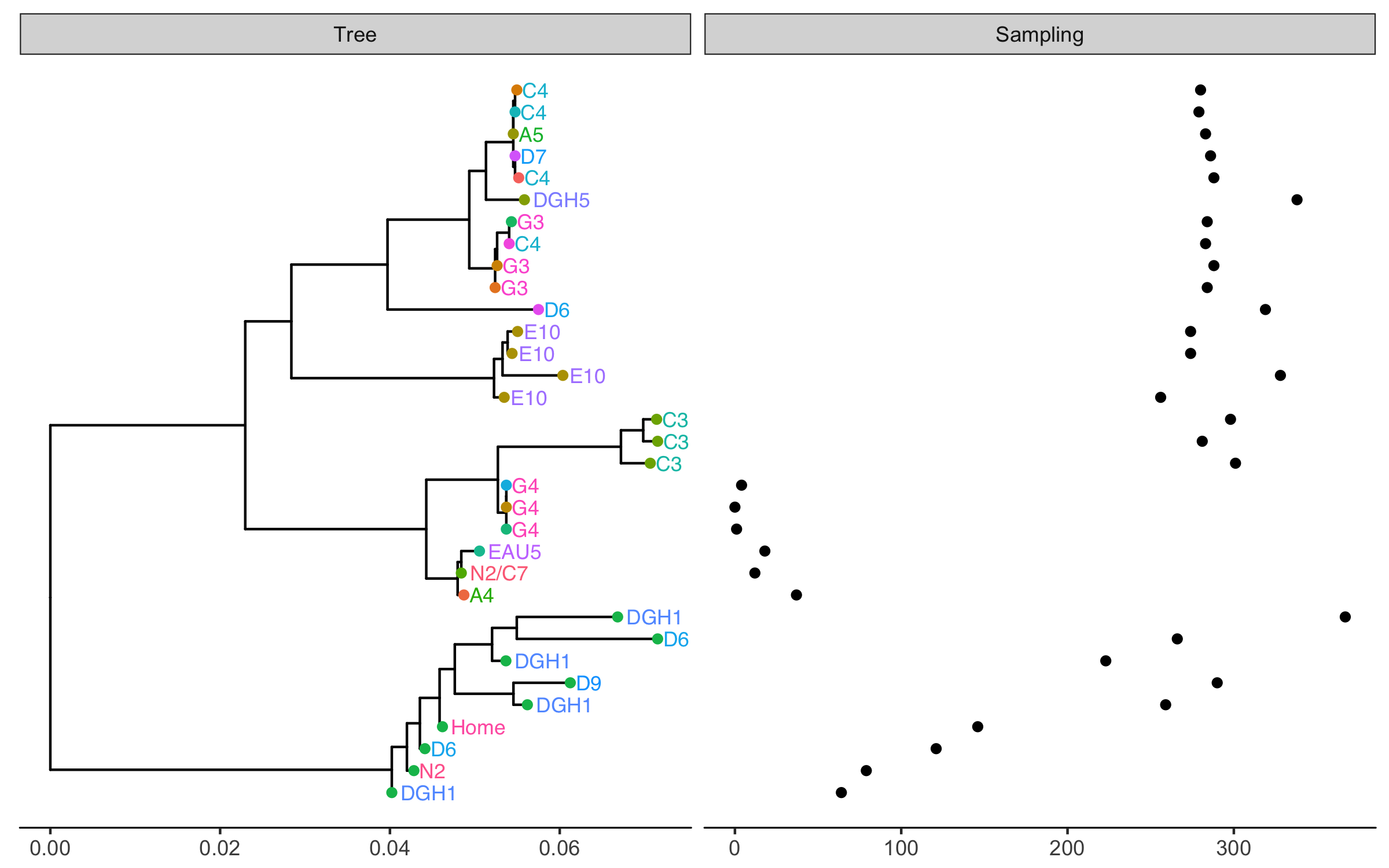
Recurrent zoonoses
- Example of influenza A H7N9 from poultry
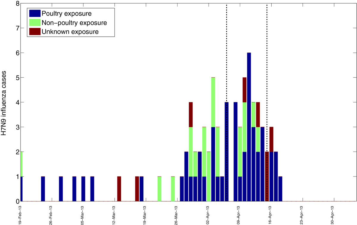
Chowell et al. BMC Medicine (2013)
Inference of introductions using case onset data only
- White and Pagano (2008) developed a method for inferring \(R_0\) and the serial interval using case onset data, based on a branching process type model
- Kucharski et al. (2014) extended this model to consider:
- A rate of introductions from outside
- Infections within the population
- This was then applied to outbreaks of influenza A H7N9
Case dynamics
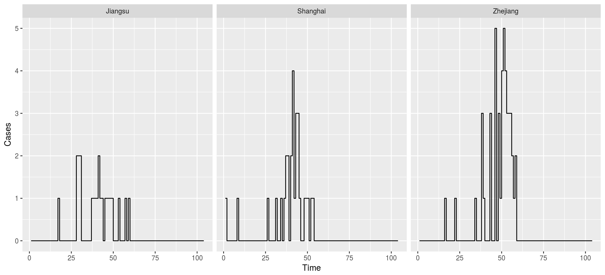
Assumptions of the modified White-Pagano
- Epidemic evolves in discrete time
- Observations are discrete, but transmission is not
- Do we count the number in the current generation as generating ‘offspring’?
- Assumes Poisson distribution of ‘offspring’
- Assumes fixed, constant serial interval
- Serial interval may change through an epidemic
Partially observed Markov model
- Instead simulate a continuous time immigration-birth-death process
- Jumps at rate \(\iota\)
- Transmissions at rate \(\lambda N\)
- Recoveries at rate \(\gamma N\)
- Use particle filtering to simulate trajectories that match the observed cases exactly
- Use MCMC to infer parameters
Inferences
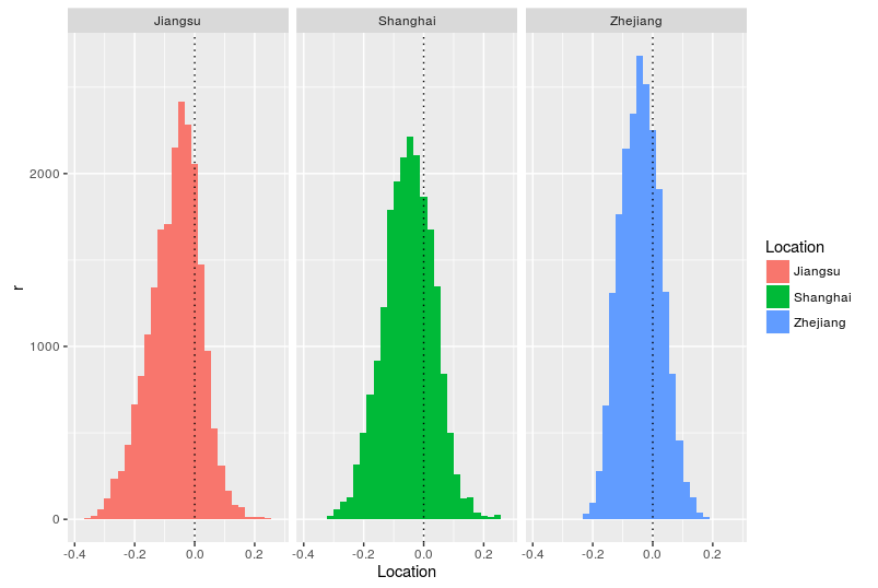
- What is the probability that \(\lambda < \gamma\)?
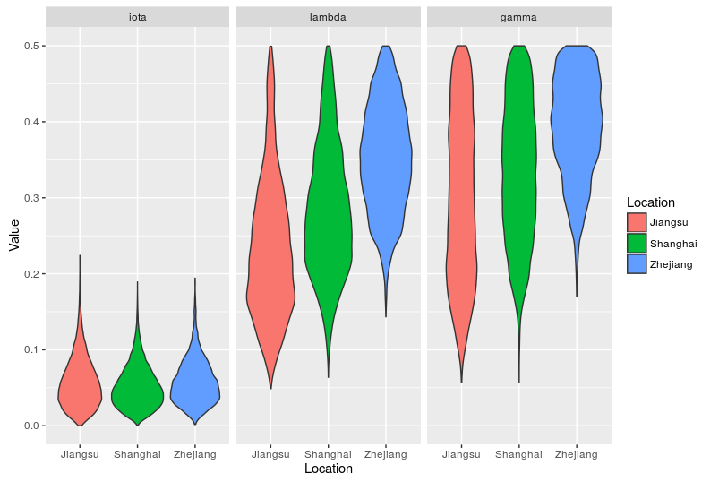
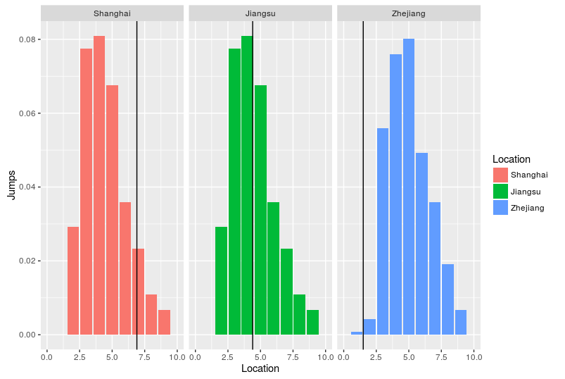
- What proportion of cases are due to spillover from a reservoir?
- How do the locations differ?
Parameter estimates
Net growth rate
Inferred number of jumps
Advantages of POMP
- More realistic mechanistic models
- Can incorporate non-independence of cases due to changing force of infection
- Application:
- Measles in South Wales, 2012-2013
South Wales measles outbreak, 2012-13
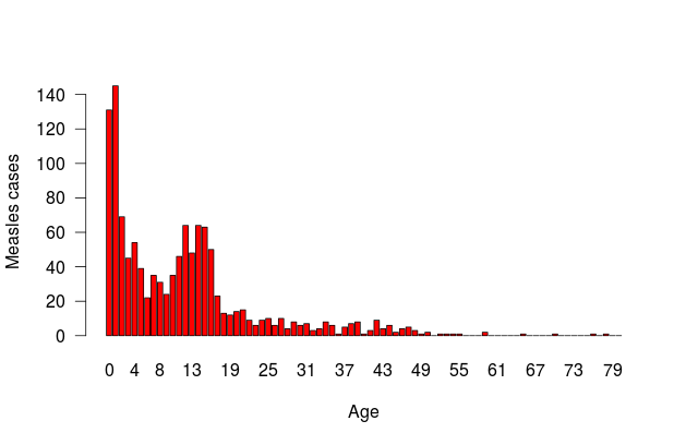
- 1212 cases of measles were reported in South Wales, 2012-13
- Largest outbreak in a high income country for many years
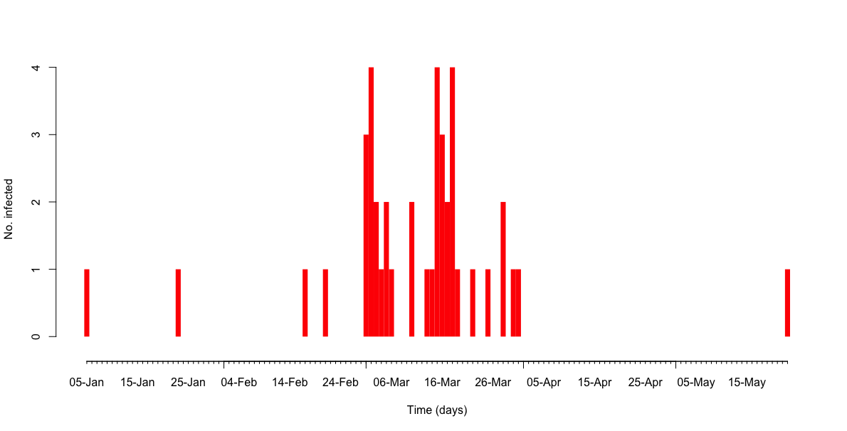
- 4 cases from schoolchildren returning from holidays
- 2 children led to the ensuing epidemic
- Multiple epidemics
- Different strain in Powys
Age distribution of cases
Spatial distribution of cases
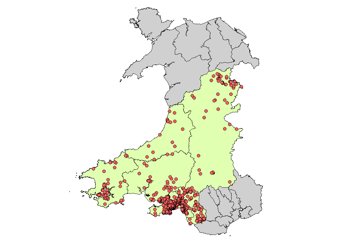
Public Health Wales, 2013
School-level dynamics
Inference of \(R_0\) and introductions
- Fitted an SEIR model
- Inference of \(R_0\) and introductions
- Fixed latent and infectious periods and population sizes
Posterior distribution
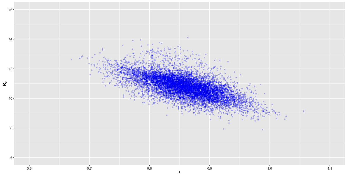
Work in progress
- Why South Wales?
- Why 2012-13?
- What were the transmission dynamics?
- \(R_0\)
- Spatial coupling
- Vaccine efficacy
- Variation between schools?
- Cause of resurgent behaviour?
- Did catch-up immunisation campaigns work?
Using sequence data to infer introductions
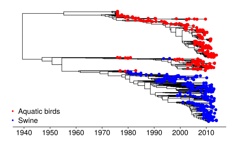
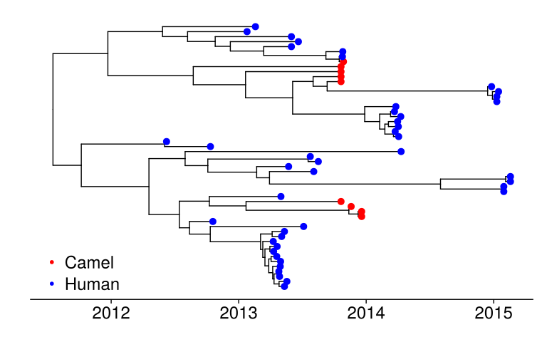
- Inferring species jumps can be performed using pathogen sequences from different species
- The phylogenetic structure of pathogen sequences depends on the rate and direction of host jumps
Low rate of host jumps
- Some pathogens jump hosts only infrequently
- e.g. influenza A H1N1 from aquatic birds to swine
High rate of host jumps
- Others jump more frequently
- e.g. MERS-CoV from camels to humans
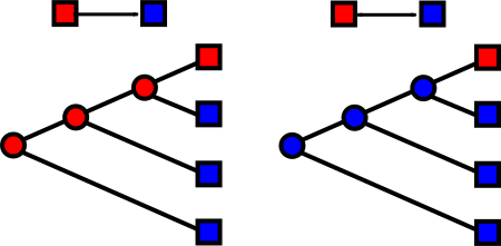
Counting the number of jumps
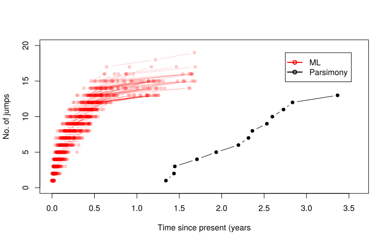
- The number of jumps is usually calculated by parsimony
- Unidirectional or bidirectional
What direction?
- The most parsimonious model may not correctly predict the direction of jumps
- For MERS-CoV in Saudi Arabia
- 5 jumps assuming human to camel
- 12 for camel to human
LASV in Sierra Leone in humans and mice
- 7 jumps from humans to mice
- 22 jumps from mice to humans
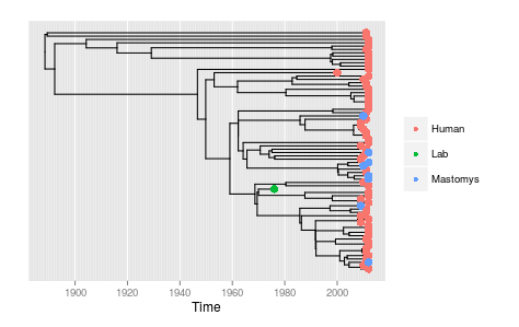
Why do trait based analyses fail?
- Biased sampling
- Samples from humans > sample from reservoir
- Samples from reservoir often taken later in time
- Just because a model permits asymmetry does not mean that it will correctly identify direction
- Unless there is simple random sampling, application of trait based models need to assume direction of transmission a priori
- Still very sensitive to sampling depth
The impact of sampling depth
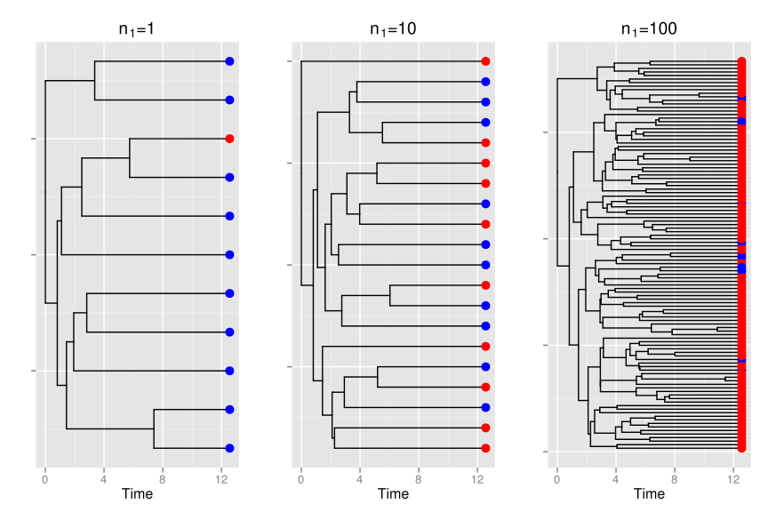
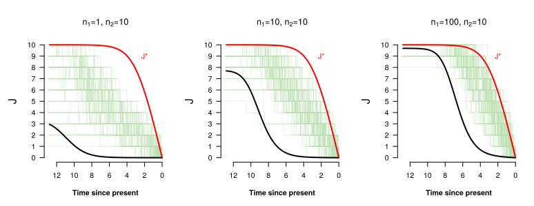
- If we have \(n_2\) sequences from our target species:
- The minimum number of host jumps is 1
- The maximum number is \(n_2\)
- This is the number of jumps in our sample (not in the population)
- The number of sampled hosts limits the number of jumps inferred
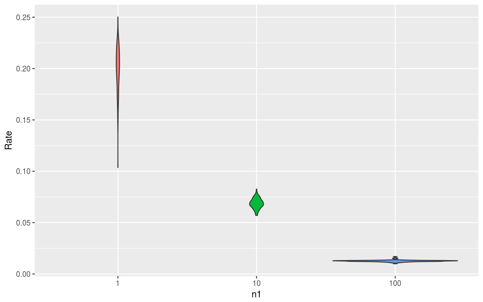
- How does the expected number of host jumps change with the number of samples from the reservoir, \(n_1\) ?
Modeling zoonotic transmission
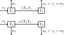
- To explore the performance of counting, we employed a simple mathematical model
- Classical ‘SIR’ compartmental model:
- Two host species
- The pathogen can jump from a ‘source’ species to a ‘target’ species
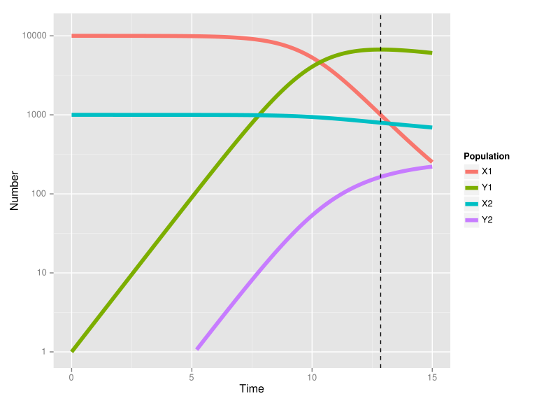
- We considered two scenarios:
- No transmission within the target species
- Transmission within the target species
Model schematic
Model dynamics
Sampling matters
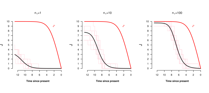
- The number of jumps in the phylogeny may be limited by the sample size from the two species
Modeling the number of jumps
- Take a sample of infected individuals in the model
- Go backwards in time
- There are three kinds of lineages
- \(A_{11}\) : lineages from the reservoir host
- \(A_{22}\) : lineages sampled from the target host that are in the target host
- \(A_{12}\) : lineages sampled from the target host that are in the reservoir
Jump equations
- \(J^*\): actual number of jumps in the sample
- \(J\): inferred number of jumps with parsimony
\[
\frac{dJ^{*}(s)}{ds} = f_{12}\frac{A_{22}}{I_2} \\\
\frac{dJ(s)}{ds} = 2 f_{11}\frac{A_{11}}{I_1}\frac{A_{12}}{I_1}+f_{12}\frac{A_{11}}{I_1}\frac{A_{22}}{I_2}
\]
Number and timing of jumps
Simple likelihood based models
- Consider the host type just as you would consider a position in a genetic sequence mutating
- Fix the root of the tree to be the source host species
- Estimate two parameters
- Reconstruct when host jumps occurred
Estimated jump rate
Reconstructed number of jumps
MERS-CoV in Saudi Arabia
Sampling issues
- In some cases, the population that an individual belongs to is not obvious
- Particularly the case for distributed contacts, and when source attribution is difficult
- Vanderbilt/China CDC study of HIV in Beijing, China
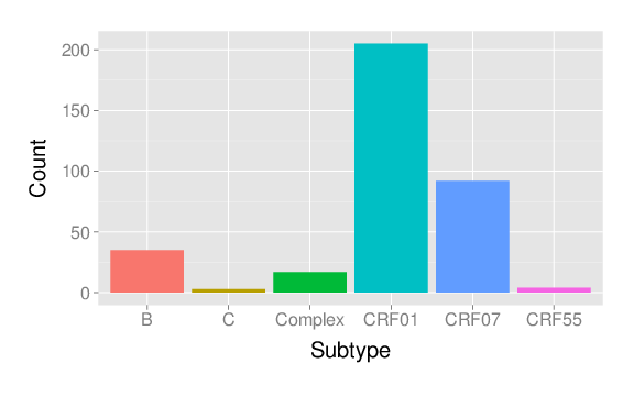
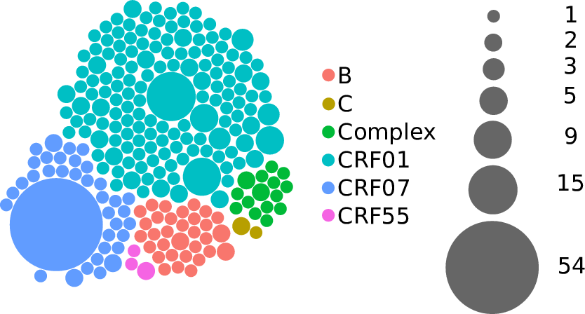
- 356 individuals with HIV-1 sequence data, who completed a behavioural questionnaire
Subtypes
Who infected whom?
- Contact data is usually not available in HIV studies
- Even when available, they are usually unreliable
- Infection with genetically similar viruses (‘clustering’) is often used as a proxy for transmission
Patterns of clustering (<1%)
Introductions or local transmission?
- If we have a focal population and a large ‘reservoir’ population, we can assume that transmission from the focal population to the reservoir is negligible
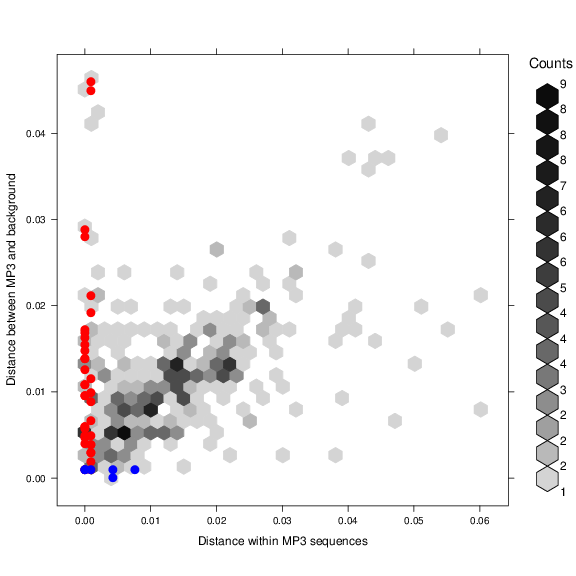
- One approach is to use database sequences as a proxy for the ‘reservoir’ population
- Distance based approaches
- Phylogeny based approaches
Minimum distances to other sequences
HIV in middle Tennessee
Subepidemics
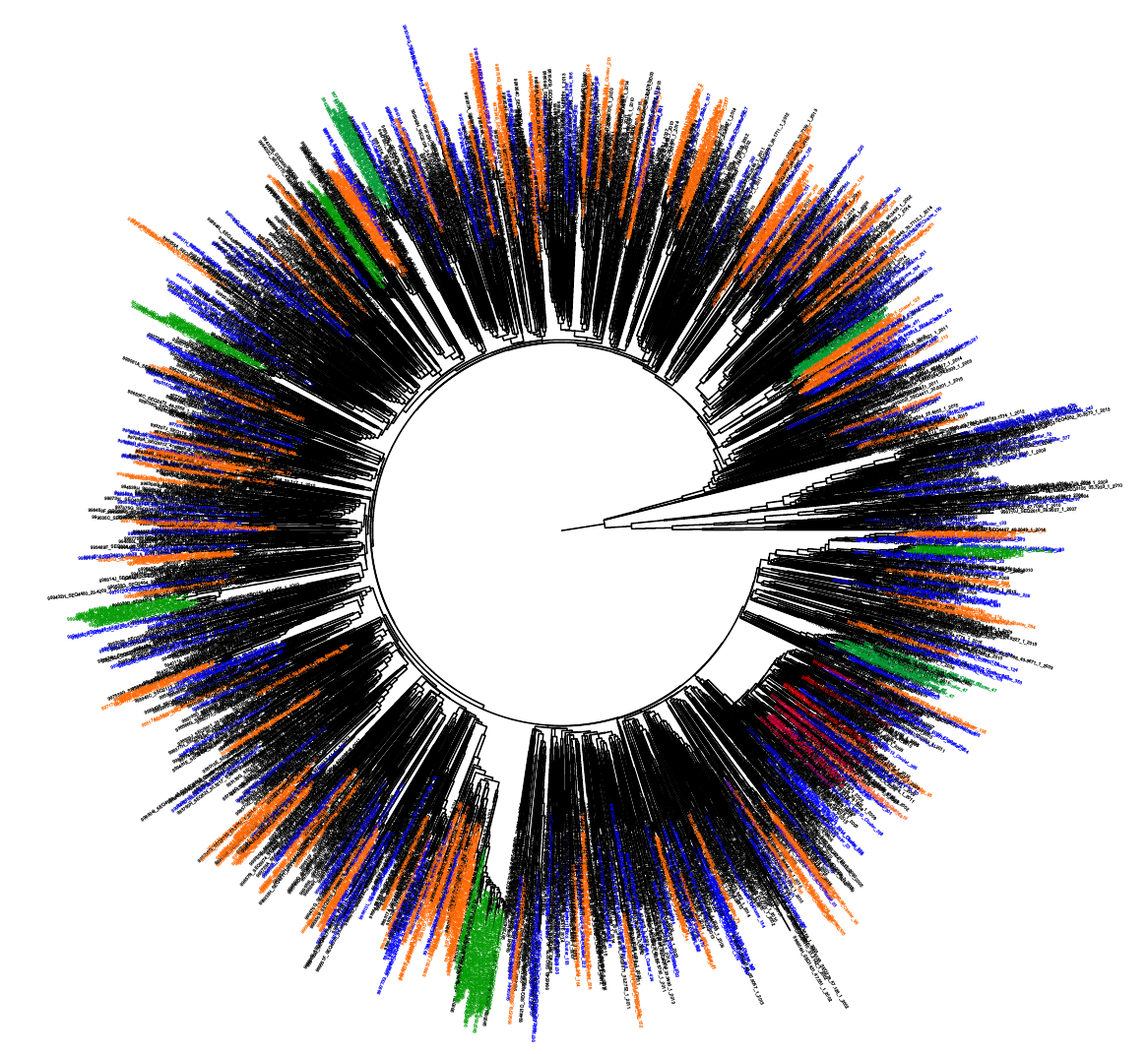
- We consider smaller subtrees:
- Slice the phylogeny at a given time
- Carve into subtrees that are monophyletic with respect to the reference sequences
- This approach is fast, and allows us to focus on phylogenies that represent ‘local’ transmission
Cluster distributions of HIV
- 2783 subtype B sequences from unique patients in middle Tennessee
- Use >100,000 reference sequences from other areas
- 931 clusters
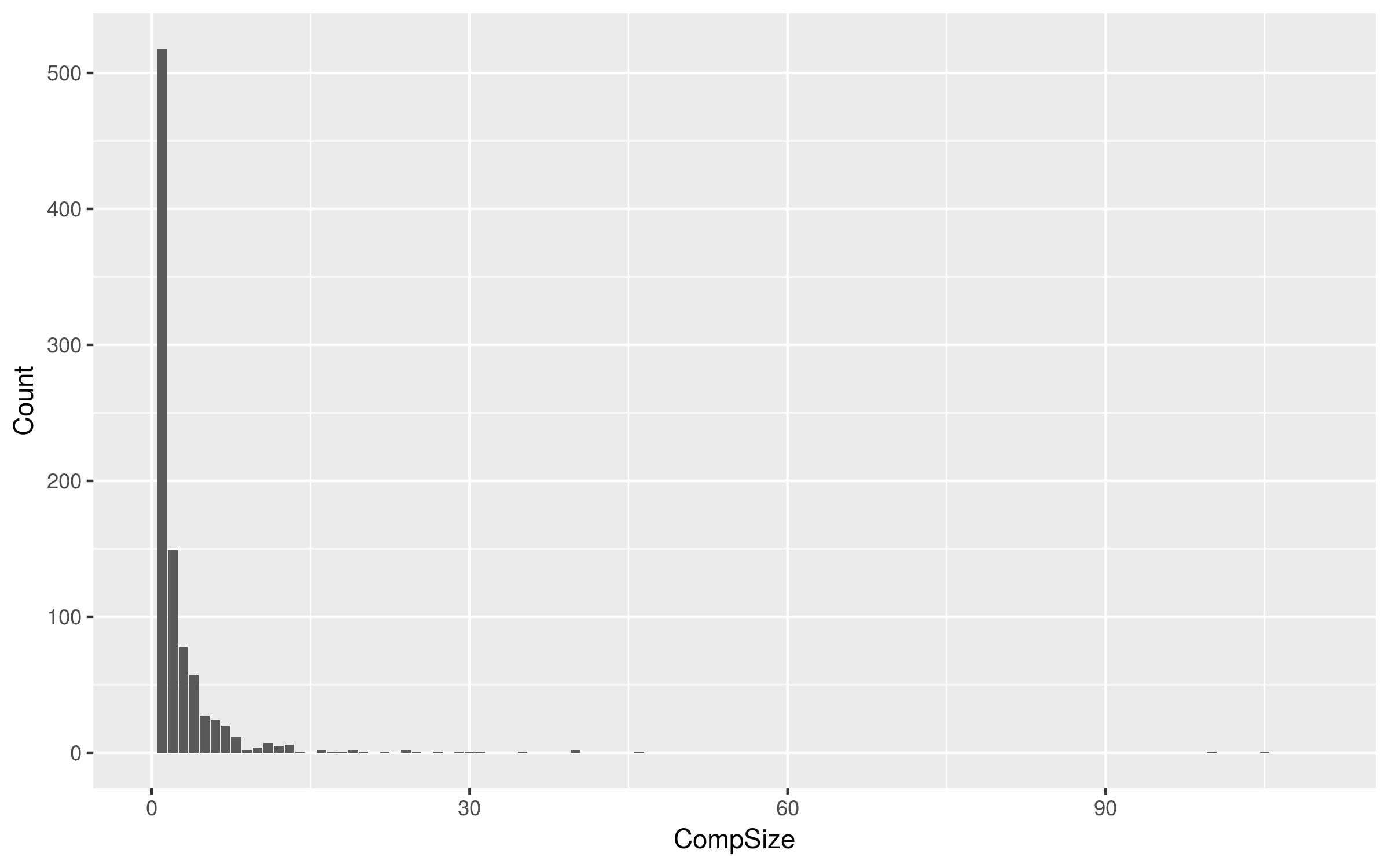
Largest monophyletic cluster
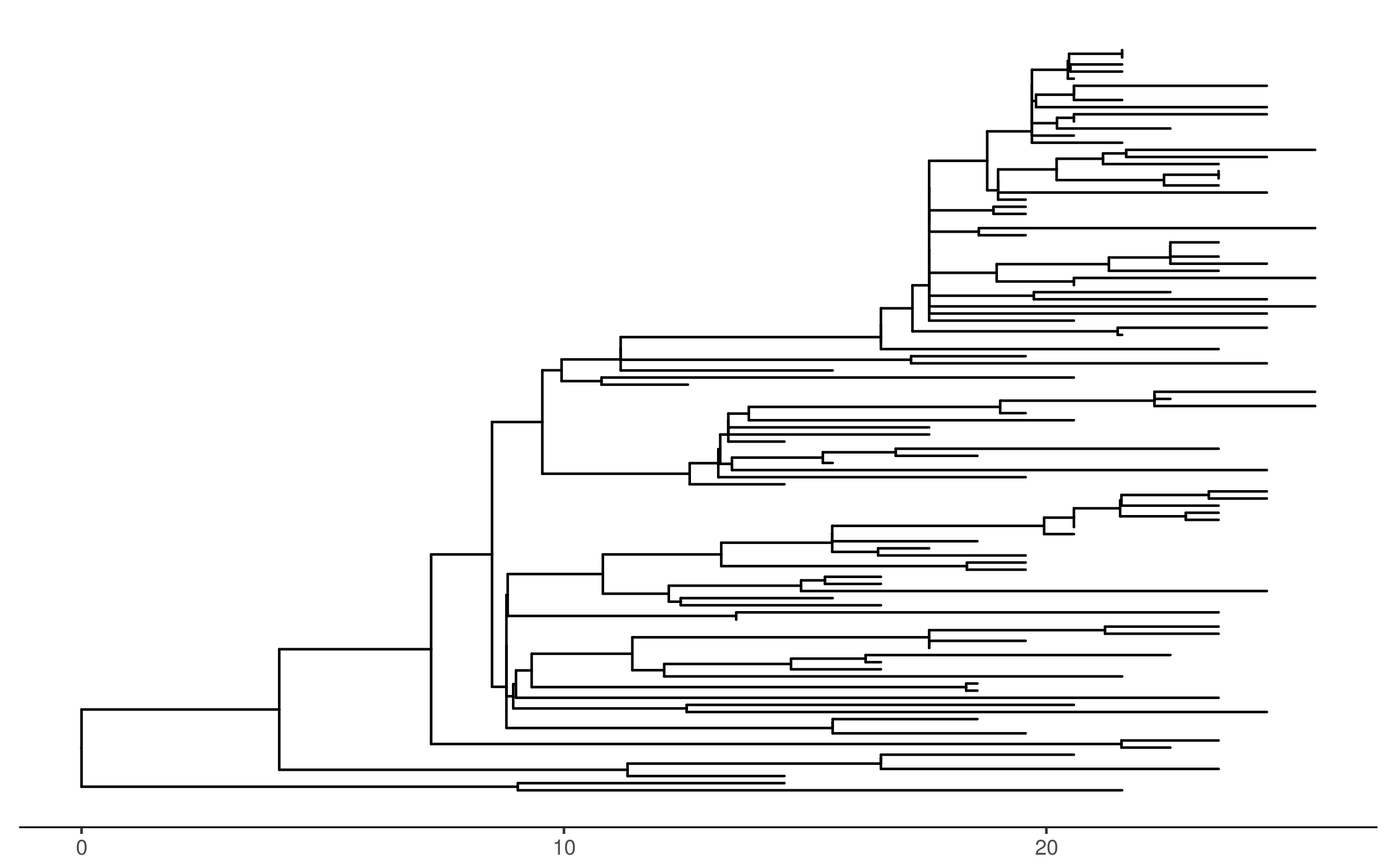
Characteristics of largest cluster
- Young
- African American
- Male, men who have sex with men
- Geographically dispersed
- Majority come from 3 ZIP3 codes
- Persisted over c. 25 years
What if we don’t know the direction?
- If we do not know the direction, we need to infer it
- Structured coalescent models are more robust to sampling biases
- Digression: coalescent models
Linking epidemiology with evolution
- Over the past ten years or so, Erik Volz and I have worked on developing a framework to convert compartmental epidemiological models into coalescent ones
- Consider a simple model of exponential growth
- \(\lambda\): growth rate
- \(\mu\): death rate
- \(I(0)\): initial number of infected individuals
\[
I(t) = I(0)e^{(\lambda-\mu)t}
\]
Stochastic model
- Infecteds, \(I\), forwards in time \(t\)
\[
\begin{array}{lllll}
\rm{Transition} & \Delta I & \rm{Rate} \cr \hline
I \rightarrow I+I & +1 & \lambda I \cr
I \rightarrow \varnothing & -1 & \mu I \cr
\end{array}
\]
Dynamics backwards in time
- Consider sampled lineages, \(A\), sampled from \(I\), backwards in time, \(s\)
- Lineages ‘coalesce’ (\(A \rightarrow A-1\)) when:
- There is an infection and
- Both lineages involved are sampled (\(A\)) rather than unsampled (\(I-A\))
\[
\begin{array}{lllll}
\rm{Transition} & \Delta A & \rm{Rate}\cr \hline
A+A \rightarrow A & -1 & \lambda I \frac{A}{I} \frac{A-1}{I-1}\cr
\end{array}
\]
Fully deterministic model
- The coalescent model is effectively a hybrid model
- Population sizes change deterministically
- Sampled lineages change stochastically
- We can make a fully deterministic model by considering differential equations for the lineages instead
- Most appropriate for large sample sizes
- Allows rapid exploration of how epidemiological parameters impact the phylogeny
\[
\begin{align}
\frac{dA(s)}{ds} & = -\lambda I \frac{A}{I}\frac{A-1}{I-1} \approx - \lambda \frac{A^2}{I}\cr
\end{align}
\]
Extensions
- More complex structured populations
- Disease stage
- Risk factors for transmission/acquisition
- Geographic location
- Host type
- More features of the tree
- Asymmetry
- Tips vs. internal branches
- Clustering
- Parameter inference
Population size from trees
- If \(I\) is the number of infecteds and \(\tau\) is the generation time, defined as the time between transmissions (per infected)
\[
N_e=I \times \tau \div 2
\] or
\[
I = 2 \times N_e \div \tau
\]
- For the exponential model:
\[
\begin{array}
\ \tau & = \frac{I}{\lambda I}\cr
& = \frac{1}{\lambda}
\end{array}
\]
Simulating the models
- Simulate the epidemiological model forwards in time to get initial conditions for the coalescent model at the present
- Simulate the coalescent model backwards in time
- Use time-varying inputs e.g. of number of infected individuals
Inference from unstructured epidemics
- We can estimate \(\nu(s)\) using a likelihood based framework, extended for censoring
- Griffiths and Tavare (1994), Pybus et al. (2000)
- The sufficient statistics are the times between coalescent or sampling events
- The likelihood of a set of intervals is the product of the partial likelihoods of each interval
- If the interval is censored, the partial likelihood of an interval \(t_i\) is:
\[
\begin{align}
P(t_i=x) & = \rm{exp}(\binom{A}{2}\Lambda(t_i))
\end{align}
\] - If the interval is uncensored:
\[
\begin{align}
P(t_i=x) & = \binom{A}{2}\nu(t_i)\rm{exp}(\binom{A}{2}\Lambda(t_i))
\end{align}
\]
where
\[
\Lambda(t)=\int_{0}^{t}\nu(s) ds
\]
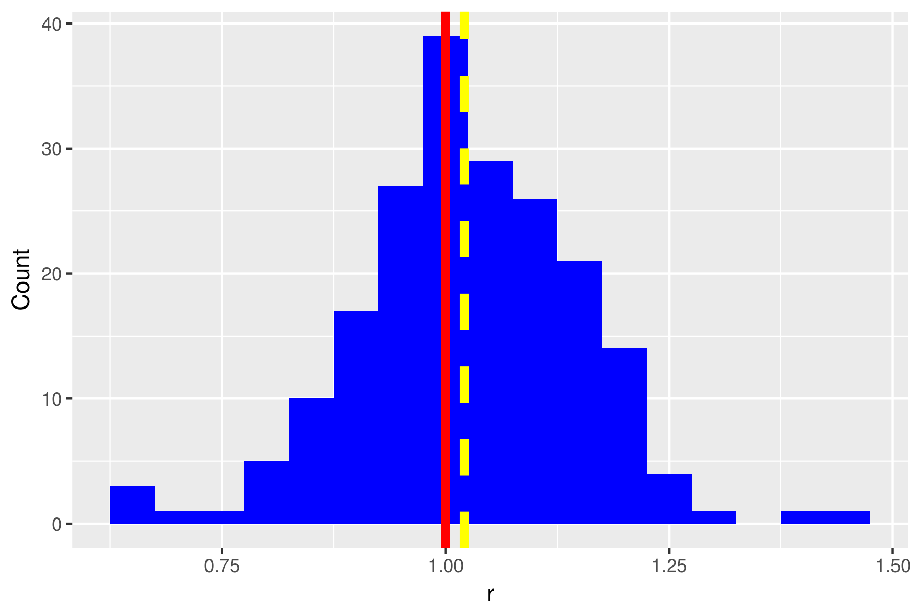
Estimates of growth rate
- Simulate 200 stochastic epidemics with \(\lambda=2\) and \(\mu=1\)
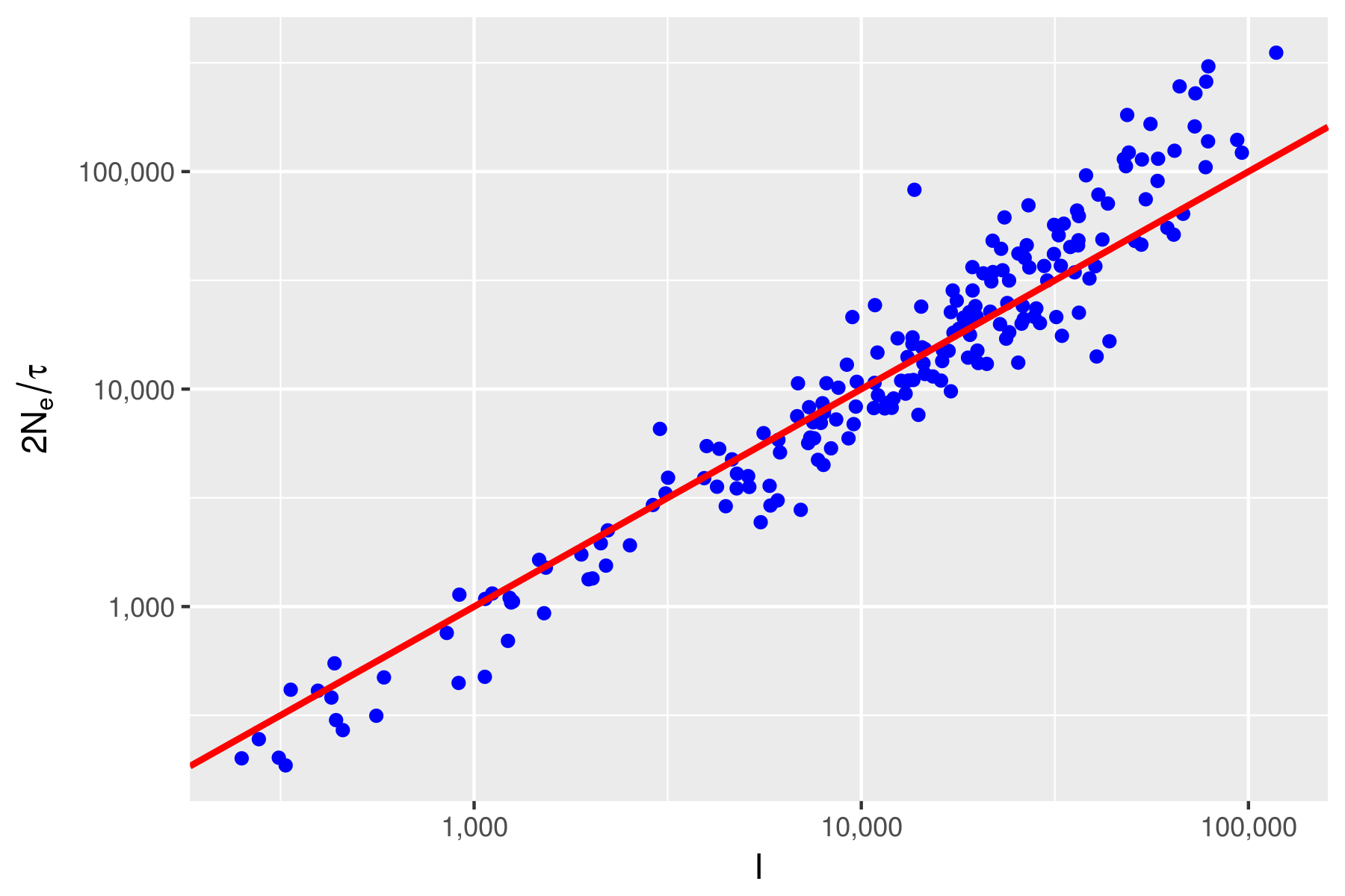
Estimates of population size
- Using our estimate of \(r=\lambda-\mu\), and assuming \(\mu=1\), we can calculate the generation time \(\tau=1/\lambda\)
- This allows us to generate estimates of the number of infected individuals
Population structure
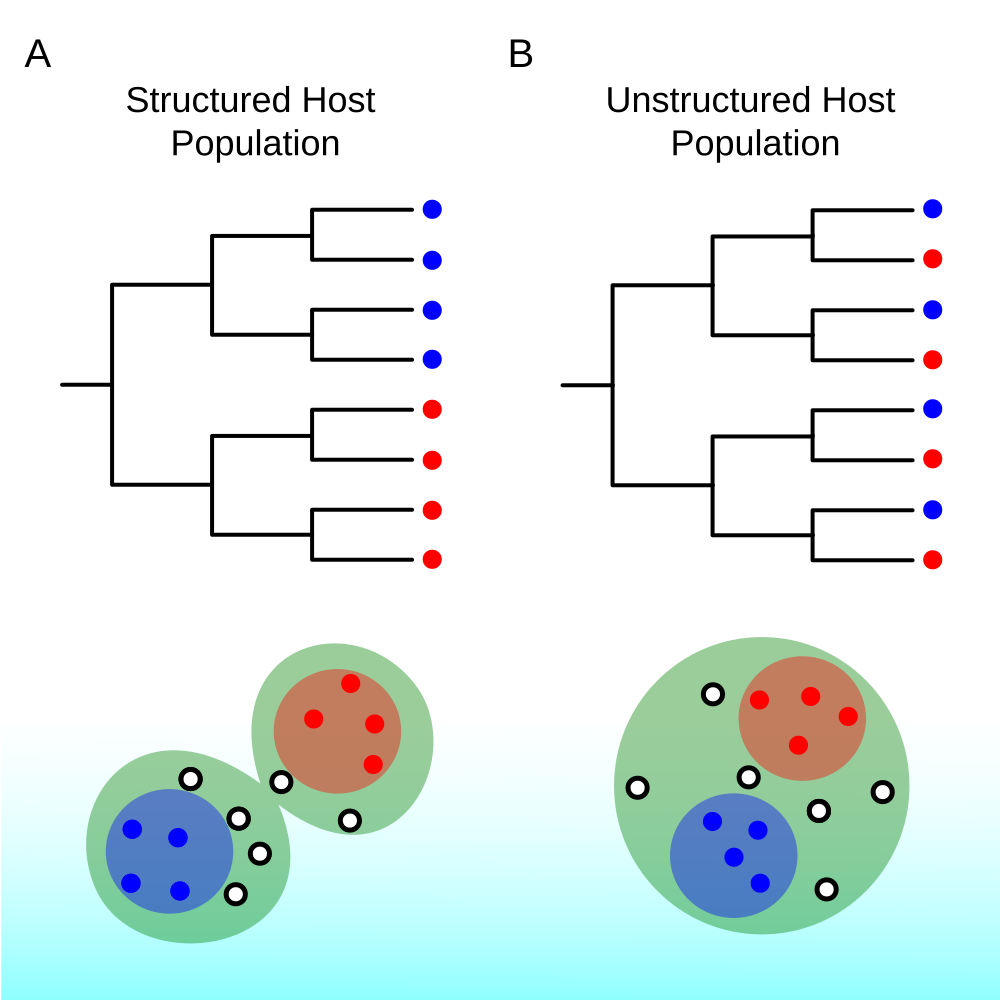
Volz et al. (2013)
Complex structured coalescent models
- Erik Volz (2012) extended the coalescent framework to consider two or more separate compartments for infected individuals
- To do this, we rewrite our epidemiological model into:
- ‘Birth’ of infected individuals
- ‘Migration’ of infected individuals in different states
- ‘Death’ of infected individuals
- All other dynamics (e.g. of susceptibles, recovered, etc.)
Inference using structured coalescent models
- In addition to considering summary statistics of a tree, we can also fit models directly to a (time-stamped) tree
- The likelihood has three components:
- The likelihood of observing a coalescent/sampling interval
- The probability of state changes along a branch
- The probability of the state immediately preceding a coalescence
Changes along a branch
- Consider \(p_{ik}\), the probability that a branch \(i\) in a phylogeny is in state \(k\) at time \(s\), measured from the present to the past
\[
\begin{align}
\frac{d p_{ik}}{ds} = & \sum_{l}^{m}\left( \frac{p_{il}}{Y_l}g_{kl}-\frac{p_{ik}}{Y_k}g_{lk}+\frac{p_{il}}{Y_l}\frac{Y_k-A_k}{Y_k}f_{kl}-\frac{p_{ik}}{Y_k}\frac{Y_l-A_l}{Y_l}f_{lk}\right)
\end{align}
\]
State of a branch after coalescence
- Consider \(p_{\alpha k}\), the probability that a parent lineage is in state \(k\) following coalescence of two daughter lineages, \(i\) and \(j\)
- Let \(\widetilde{\lambda_{ij}}\) be the coalescence rate between lineages \(i\) and \(j\), summed over all states of \(i\) and \(j\)
\[
\begin{align}
p_{ \alpha k} = \frac{1}{\widetilde{\lambda_{ij}}}\sum_{l}^{m} \frac{f_{kl}}{Y_k Y_l}\left(p_{ik}p_{jl}+p_{il}p_{jk}\right)
\end{align}
\]
Coalescence rate between branches
\[
\begin{align}
\widetilde{\lambda_{ij}} = \sum_{k}^{m} \sum_{l}^{m} f_{kl} \frac{p_{ik}p_{jl}+p_{il}p_{jk}}{Y_k Y_l}
\end{align}
\]
Approximations
- Assembling the three components into a likelihood results in a very large system of differential equations
- Approximations are made
- Solve for the dynamics of the total number of ancestors of each type, \(A_k\), rather than the state of each lineage
- Solving \(m\) representative state vectors in each internode interval
- This allows complex models to be fitted in a reasonable amount of time
Simplification
- In SIR-type compartmental models, the coalescent rate depends on the transmission rate and the sampling fraction
- We fix the actual population size at a nominal value so as to infer the effective population size
- For a structured epidemic, we infer effective population sizes and migration rates using maximum (pseudo)likelihood
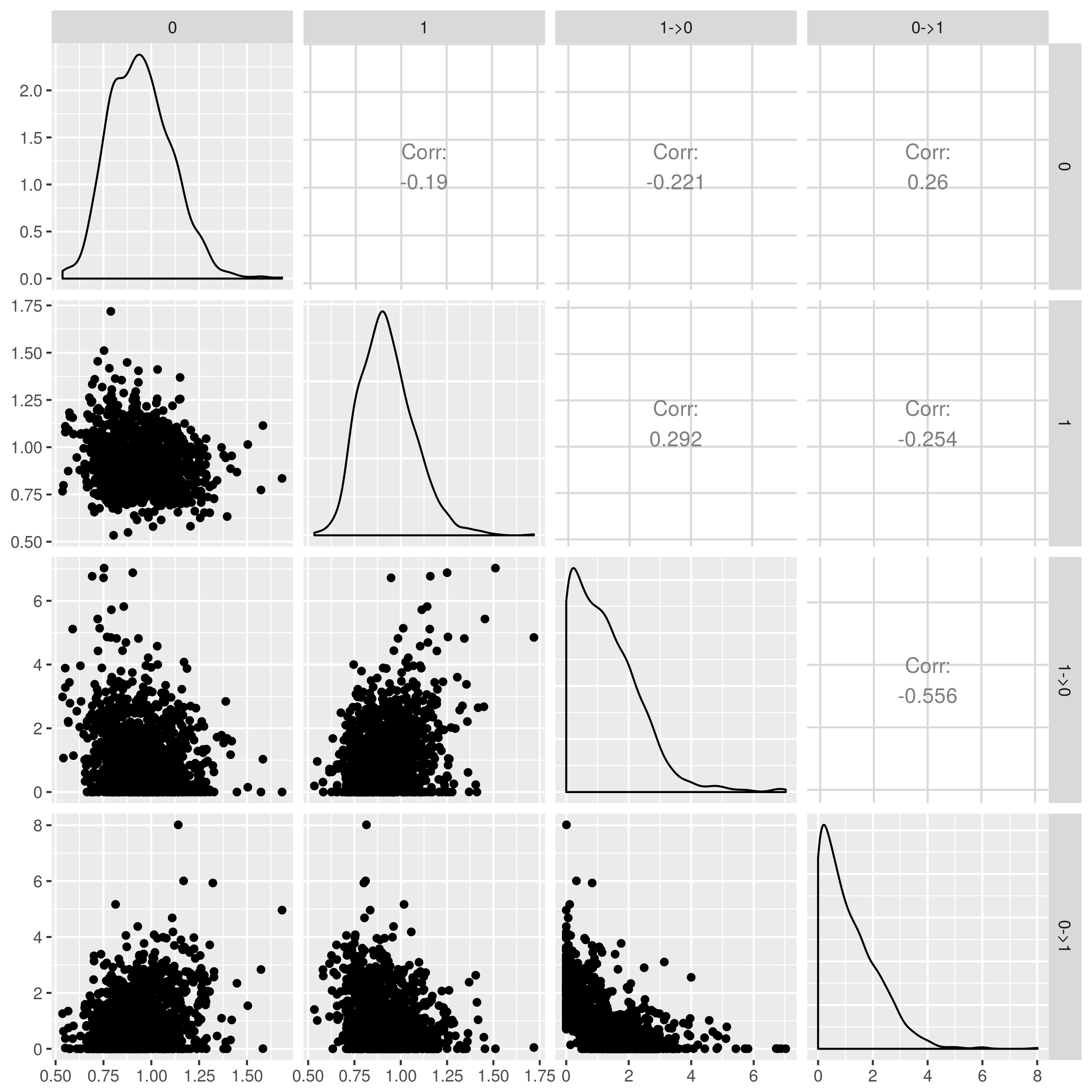
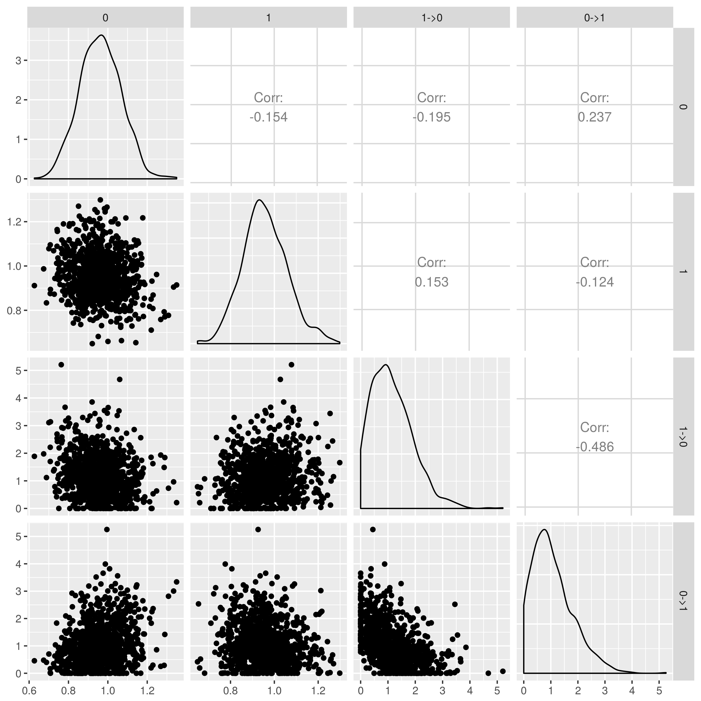
Simulations
- Consider two populations with migration between them
- Two ‘effective population sizes’
- Two migration rates
- Can we recover the parameter values?
- Can we correctly infer the ancestral states?
Parameter estimates (n=50/deme)
Parameter estimates (n=100/deme)
Fit of the MERS dataset
Estimated effective sizes and rates:

camel        8.436281e+00
human        1.517501e+00
human->camel 1.332137e-05
camel->human 3.019339e+00
State at the root of the tree
    camel        human
        1 1.030951e-10
    camel     human
0.3159066 0.6840934
Simulated DI model
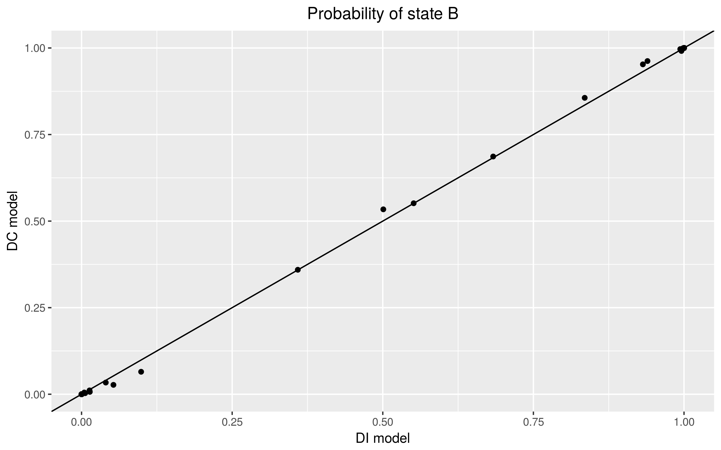
MERS-CoV
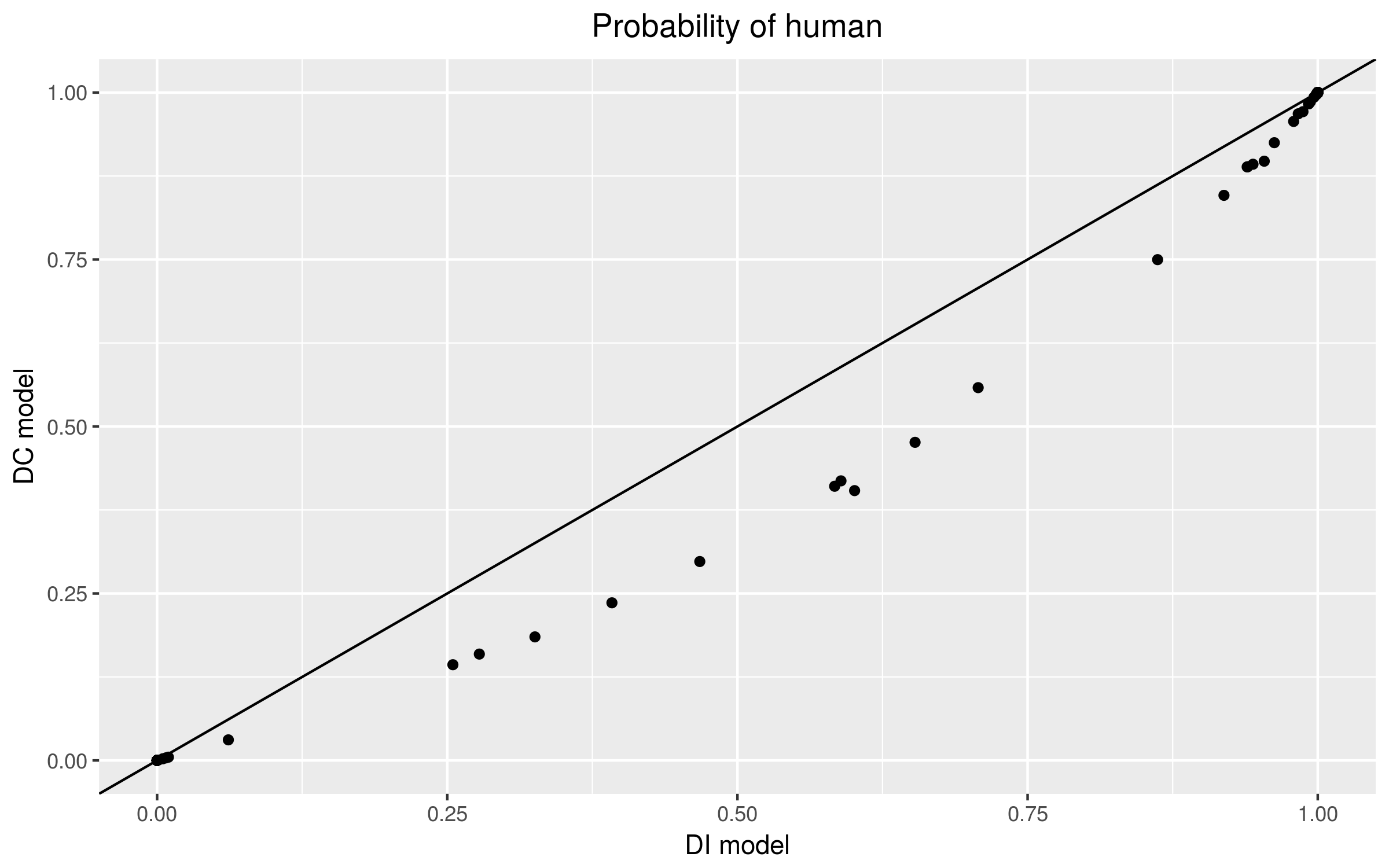
- The model fit (lnL) is the same under the DC and DI models
- Population sizes are v. similar
- Absolute size of migration rates differ: given the lack of identifiability, this is not surprising
- Ancestral reconstructions differ
Comparison of ancestral reconstructions
Digression: sources within a population
- Even within a population, there are those who have not (yet) contributed to onward transmission
- Can we infer who has and who has not infected other individuals?
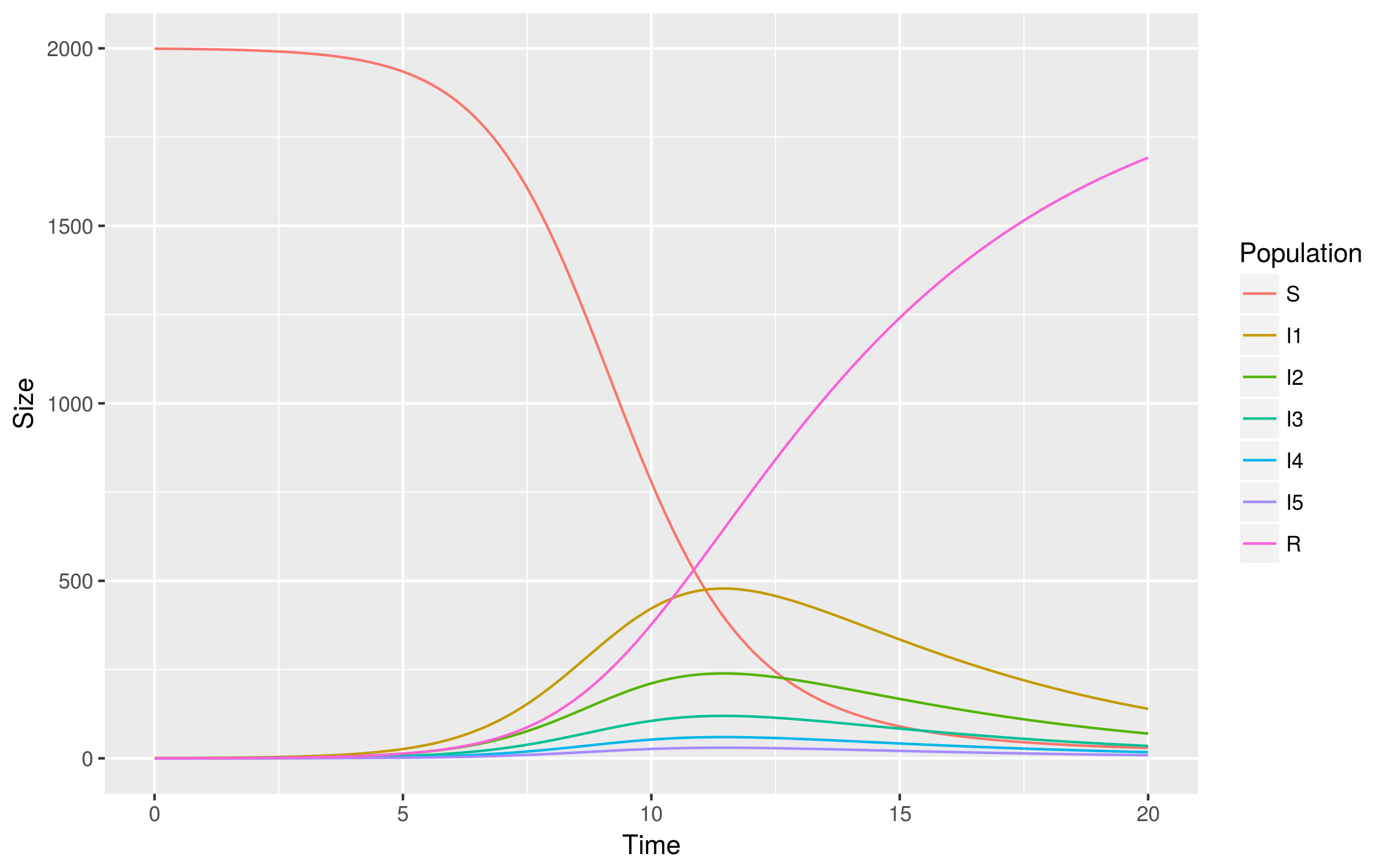
Counting infections
- Let us consider a simple ‘SIR’ type epidemiological model in which we count the number of times an individual has infected another
- No intrinstic differences between individuals
- In the absence of infection, what is the degree of the transmission network?
A model
\[
\begin{align}
\frac{dS}{dt} & = -\beta S \Sigma_i I_i\cr
\frac{dI_1}{dt} & = \beta S \Sigma_i I_i - \gamma I_1 - \beta S I_1\cr
\frac{dI_i}{dt} & = \beta S I_{i-1} - \gamma I_i - \beta S I_i\cr
\frac{dI_N}{dt} & = \beta S I_{N-1} - \gamma I_N\cr
\end{align}
\]
Dynamics
Proportions
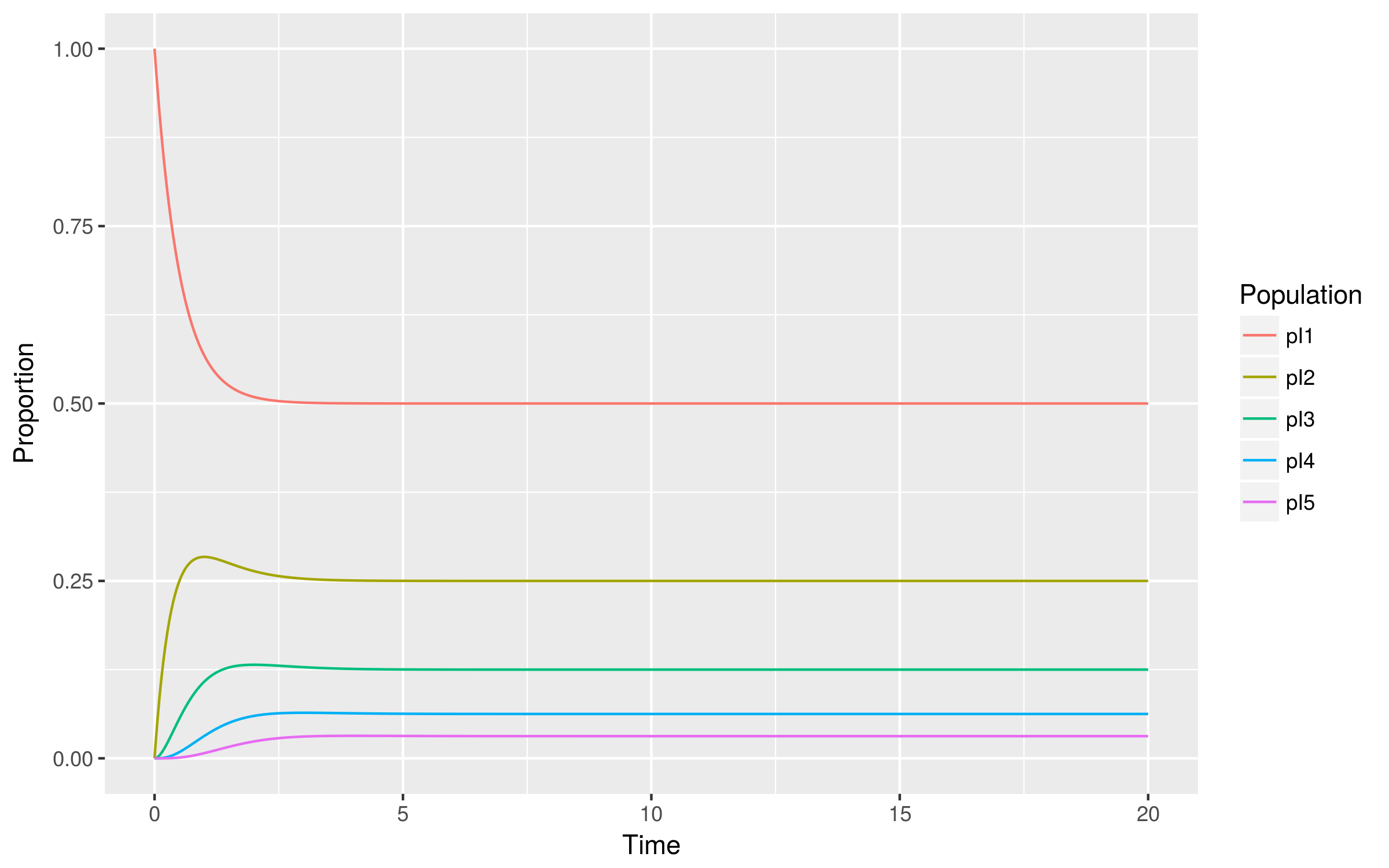
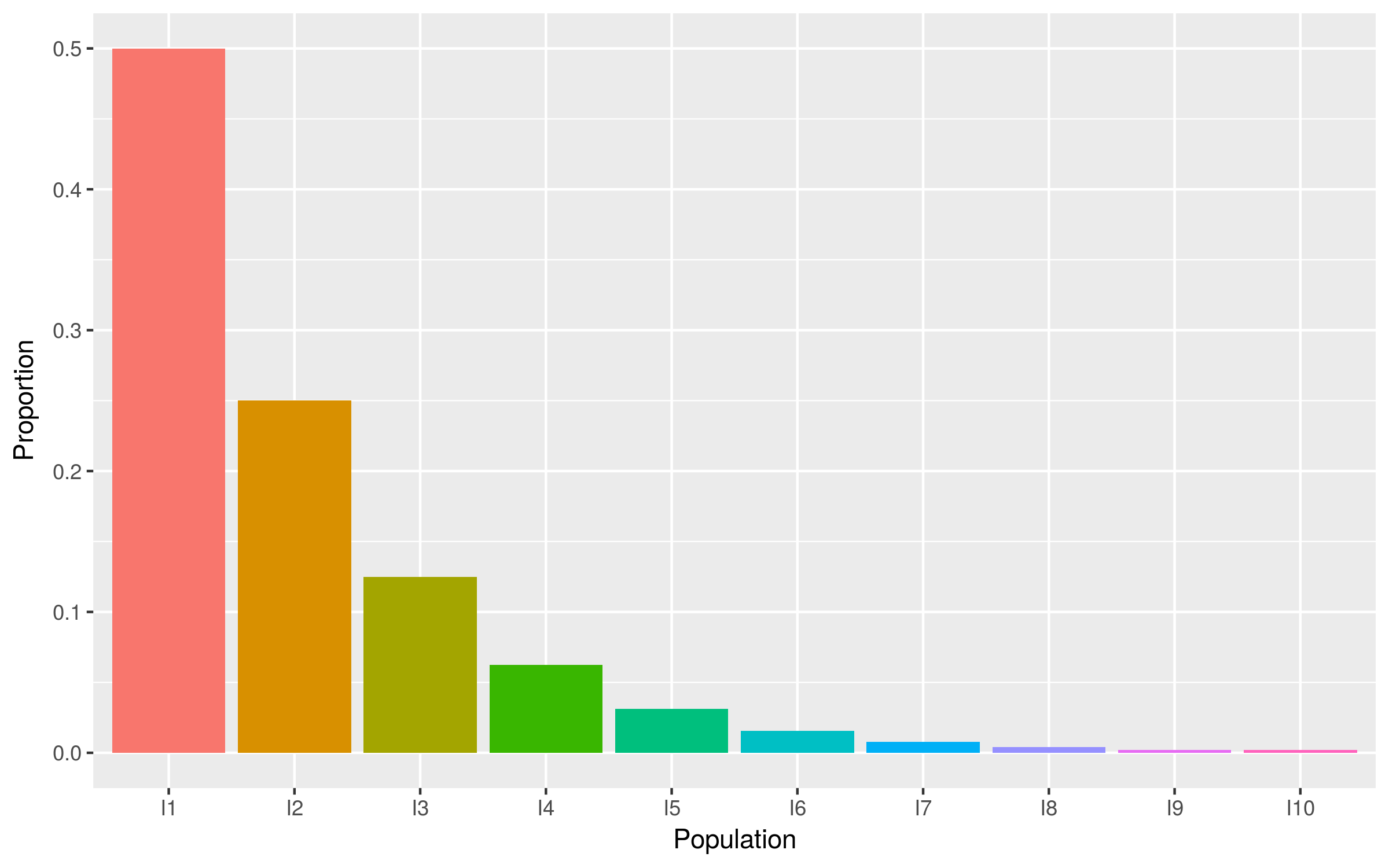
Degree distribution is geometric
- Half of individuals at any one time have not (yet) infected anyone
Phylodynamic modeling
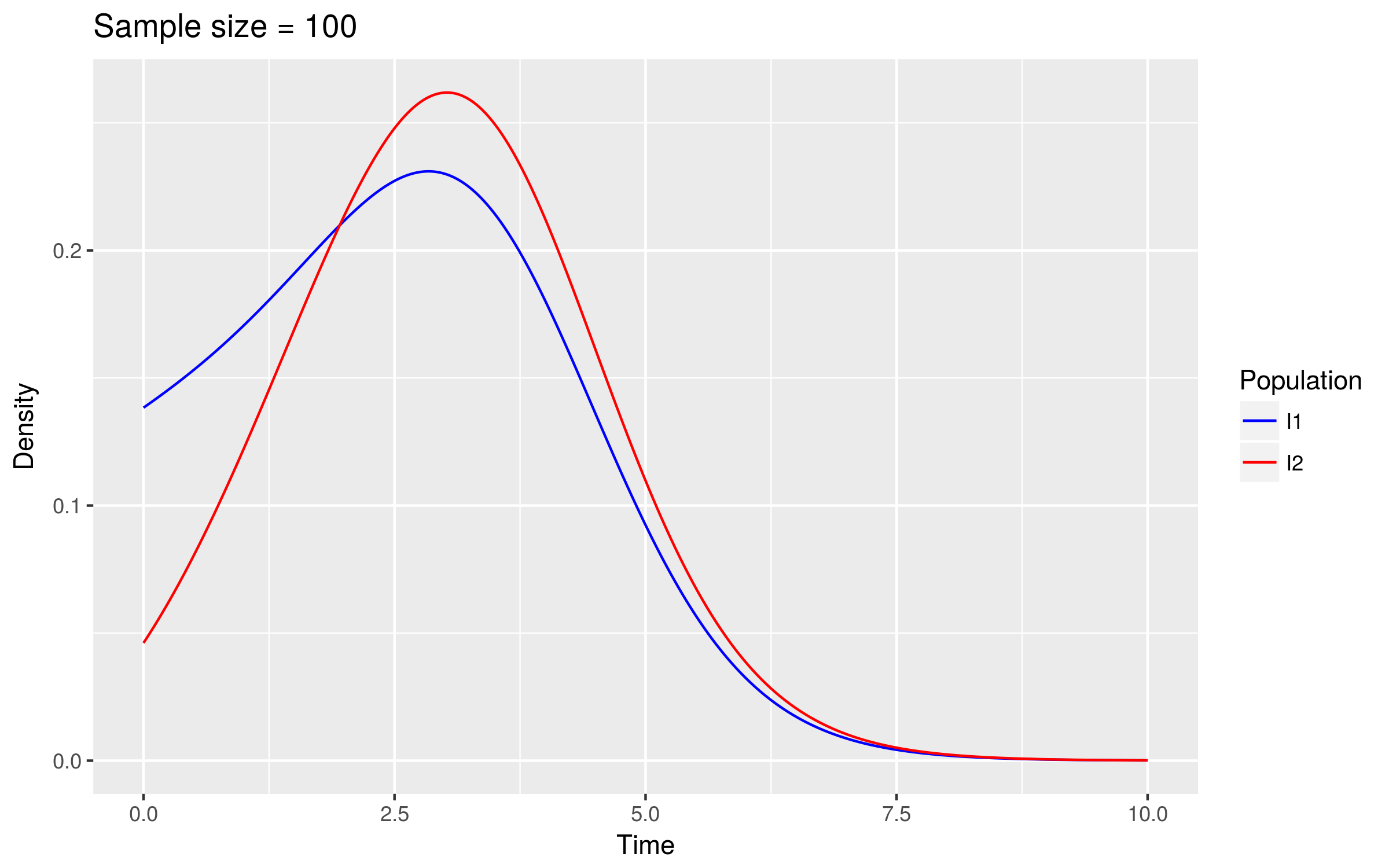
- Divide individuals up into those who did and did not infect others
- Build a phylodynamic model backwards in time and compare the evolutionary dynamics of the two groups
Tip lengths differ (high sample fraction)
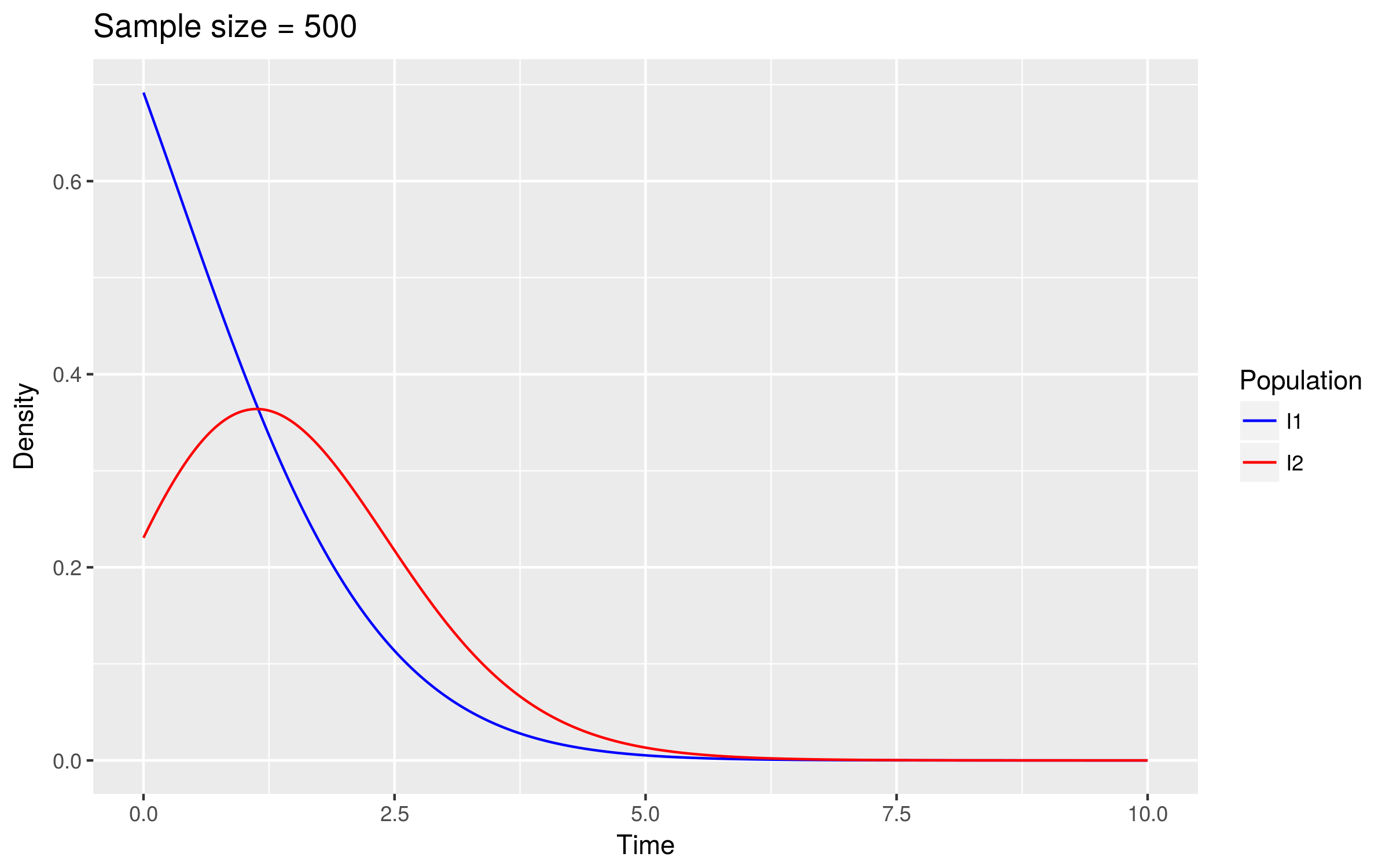
Tip lengths similar (low sample fraction)
Using tip lengths
- Ideally, we would assign a latent variable to each individual depending on their (hidden) number of infectees
- Inference using the full phylogeny can be very computationally intensive
- The previous modeling suggested that tip lengths may be informative of infection
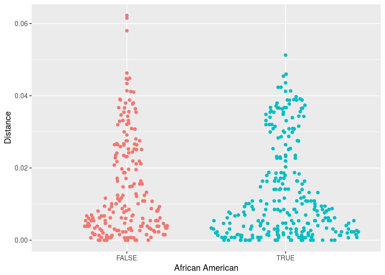
- One simple approach we have used is to calculate the distance to the nearest sequence
- Closer sequences = more clustering
- This approach does not involve choosing a threshold number of SNPs
HIV in middle Tennessee
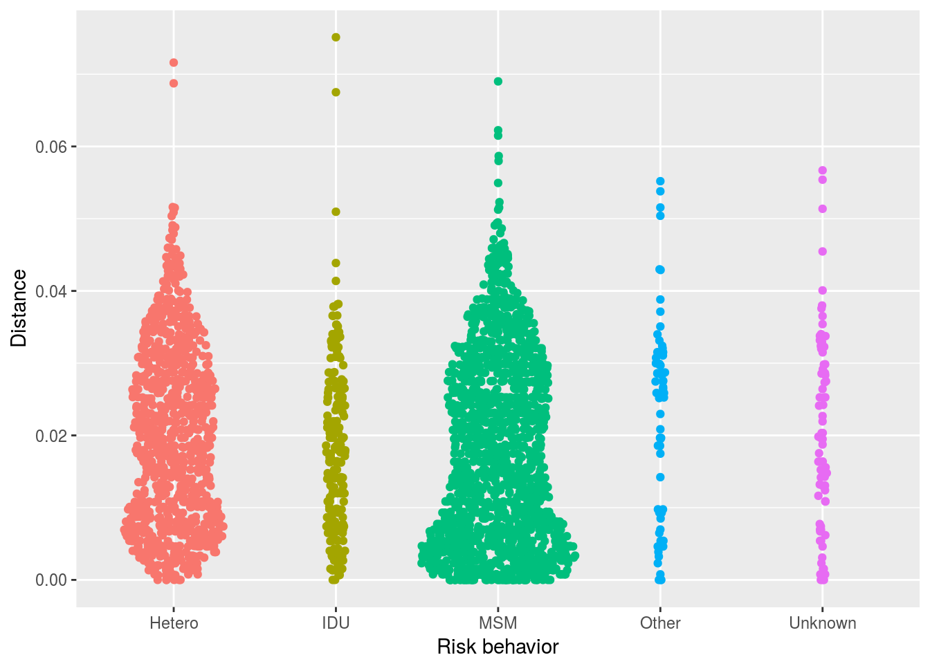
Clustering by age
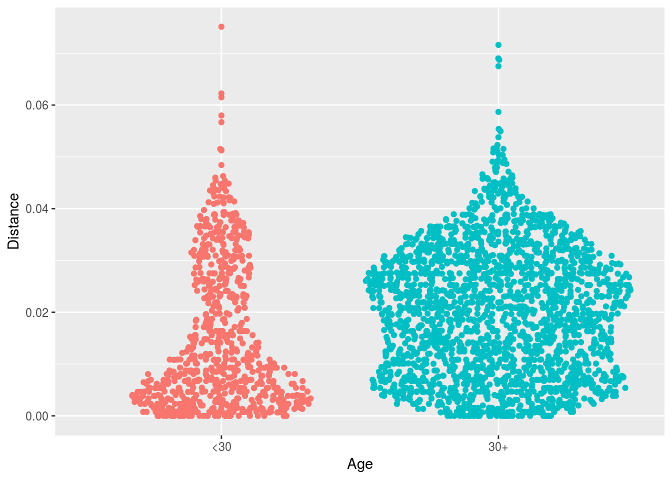
Clustering by race among young MSM
Conclusions
- Case onset data can provide some information on introductions
- Especially when cases are rare
- Data on potential sources of infection are useful (even if noisy)
- Sampling biases are important to consider
- May be able to detect introductions on the basis of how they affect tree structure
Acknowledgements
- University of Cambridge
- Imperial College London
- Swansea University
- Vanderbilt
- Yale
- Han-Zhu Qian
- Sten Vermund
- China CDC
- Princeton
 sdwfrost@gmail.com
 @sdwfrost
 http://github.com/sdwfrost